On next week’s episode of the ‘Are You Entertained?’ podcast, we’re going to be analyzing the latest generation’s guilty pleasure- the music of the ’00s. Our Data Scientists have poured through Billboard chart data to analyze what made a hit soar to the top of the charts, and how long they stayed there. Tune in next week for an awesome exploration of music and data as we continue to address an omnipresent question in the industry- why do we like what we like?
Project Summary
For this project, I imported and cleaned the data, and computed:
- The most popular artists in 2000
- The #1 songs in songs in 2000
- The time it takes for songs to reach #1, compared to the entire list
Importing Data
First we’ll look at the data to see what features are available and to see which type conversions might be necessary.
year                 int64
artist.inverted     object
track               object
time                object
genre               object
date.entered        object
date.peaked         object
x1st.week            int64
x2nd.week          float64
x3rd.week          float64
x4th.week          float64
x5th.week          float64
x6th.week          float64
x7th.week          float64
x8th.week          float64
dtype: object
   year      artist.inverted                                  track  time  \
0  2000      Destiny's Child               Independent Women Part I  3:38
1  2000              Santana                           Maria, Maria  4:18
2  2000        Savage Garden                     I Knew I Loved You  4:07
3  2000              Madonna                                  Music  3:45
4  2000  Aguilera, Christina  Come On Over Baby (All I Want Is You)  3:38

  genre date.entered date.peaked  x1st.week  x2nd.week  x3rd.week     ...      \
0  Rock   2000-09-23  2000-11-18         78       63.0       49.0     ...
1  Rock   2000-02-12  2000-04-08         15        8.0        6.0     ...
2  Rock   1999-10-23  2000-01-29         71       48.0       43.0     ...
3  Rock   2000-08-12  2000-09-16         41       23.0       18.0     ...
4  Rock   2000-08-05  2000-10-14         57       47.0       45.0     ...

   x67th.week  x68th.week  x69th.week  x70th.week  x71st.week  x72nd.week  \
0         NaN         NaN         NaN         NaN         NaN         NaN
1         NaN         NaN         NaN         NaN         NaN         NaN
2         NaN         NaN         NaN         NaN         NaN         NaN
3         NaN         NaN         NaN         NaN         NaN         NaN
4         NaN         NaN         NaN         NaN         NaN         NaN

   x73rd.week  x74th.week  x75th.week  x76th.week
0         NaN         NaN         NaN         NaN
1         NaN         NaN         NaN         NaN
2         NaN         NaN         NaN         NaN
3         NaN         NaN         NaN         NaN
4         NaN         NaN         NaN         NaN

[5 rows x 83 columns]
Preparing Data
As a matter of preference, let’s rearrange the artist names column so that it reads first_name last_name, and rename the column to something more intuitive. Also, we’ll want to convert date.entered and date.peaked so we can perform calculations on those values. Take a look at the datetime columns to see how they’re written (which could affect the arguments in pd.to_datetime()):
data[['date.entered', 'date.peaked']] = data[['date.entered', 'date.peaked']].apply(pd.to_datetime, yearfirst = True, errors = 'coerce')

print(data[['date.entered', 'date.peaked']].head().dtypes)
date.entered    datetime64[ns]
date.peaked     datetime64[ns]
dtype: object
Analysis
First, which artists had the most songs on the billboard?
songs_on_the_billboard = data['artist_name'].value_counts()
songs_on_the_billboard[0:10]
Jay-Z                  5
Whitney Houston        4
The Dixie Chicks       4
The Backstreet Boys    3
Sisqo                  3
Toni Braxton           3
Britney Spears         3
LeAnn Rimes            3
Kelly Price            3
SheDaisy               3
Name: artist_name, dtype: int64
It appears that Jay-Z was the most popular overall, but let’s calculate his z score and p value to be sure that it’s not from random chance:
z = (5 - songs_on_the_billboard.mean()) / songs_on_the_billboard.std()
z
5.087836432701593
Jay-Z’s z-score of $5\sigma$ means that $p < 0.0001$, which means his song count is statistically significant.
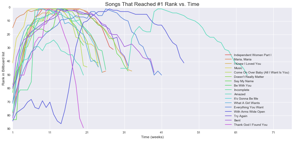
Songs that made it to #1
# Select the columns that represent the weekly scoring, then select the rows that held the #1 spot
held_top_spot = data[data.iloc[:, 7:].apply(min, axis = 1) == 1]

print(held_top_spot[['track', 'artist_name']])

held_top_spot['genre'].value_counts()
                                    track         artist_name
0                Independent Women Part I     Destiny's Child
1                            Maria, Maria             Santana
2                      I Knew I Loved You       Savage Garden
3                                   Music             Madonna
4   Come On Over Baby (All I Want Is You)  Christina Aguilera
5                   Doesn't Really Matter               Janet
6                             Say My Name     Destiny's Child
7                             Be With You    Enrique Iglesias
8                              Incomplete               Sisqo
9                                  Amazed            Lonestar
10                       It's Gonna Be Me              N'Sync
11                      What A Girl Wants  Christina Aguilera
12                    Everything You Want    Vertical Horizon
13                    With Arms Wide Open               Creed
14                              Try Again             Aaliyah
15                                   Bent     matchbox twenty
16                  Thank God I Found You        Mariah Carey


Rock       15
Country     1
Latin       1
Name: genre, dtype: int64
However the genre data needs to be manually corrected since some songs are miscategorized. For example:
| track | artist_name | genre | |
|---|---|---|---|
| 17 | Breathe | Faith Hill | Rap |
| 190 | Let's Make Love | Faith Hill | Rap |
Time to top
How long does it take for the top songs to reach the #1 spot?
# Time to top refers to the songs that reached #1
time_to_top = (held_top_spot['date.peaked'] - held_top_spot['date.entered']).dt.days
time_to_top.describe()
count     17.000000
mean      94.705882
std       60.678213
min       35.000000
25%       56.000000
50%       84.000000
75%       91.000000
max      273.000000
dtype: float64
Let’s compare this to the entire dataset:
# Time to peak calculates over all songs
time_to_peak_all = (data['date.peaked'] - data['date.entered']).dt.days
time_to_peak_all.describe()
count    317.000000
mean      52.246057
std       40.867601
min        0.000000
25%       21.000000
50%       49.000000
75%       70.000000
max      315.000000
dtype: float64
Do these data have statistically different means? We can try performing Welch’s t-test, but first we need to see if the datasets have normal distributions.
sns.distplot(time_to_top, norm_hist = True, bins = 15, label = 'Songs that reached #1', kde = False)
sns.distplot(time_to_peak_all, norm_hist = True, bins = 20, label = 'All songs', kde = False)

# Plot formatting
sns.set_palette(sns.color_palette(palette = 'hls', n_colors = 2))
plt.xlim(xmin = 0)
plt.legend()

sns.plt.show()
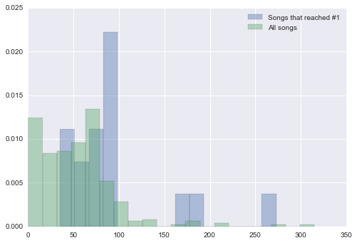
Neither data set appears to be normally distributed, as they are both positively skewed. Therefore we cannot technically apply a two-sample t-test to determine if the mean values are statistically separate. But when we run Welch’s t-test, we find:
peak_vs_top_t_statistic = scipy.stats.ttest_ind(time_to_top, time_to_peak_all, equal_var = False)
print("t-statistic: {}\np-value: {}".format(peak_vs_top_t_statistic[0].round(3), peak_vs_top_t_statistic[1].round(3)))
t-statistic: 2.851
p-value: 0.011
This would have let us reject the null hypothesis and state that the songs that reached #1 are statistically different from other songs.
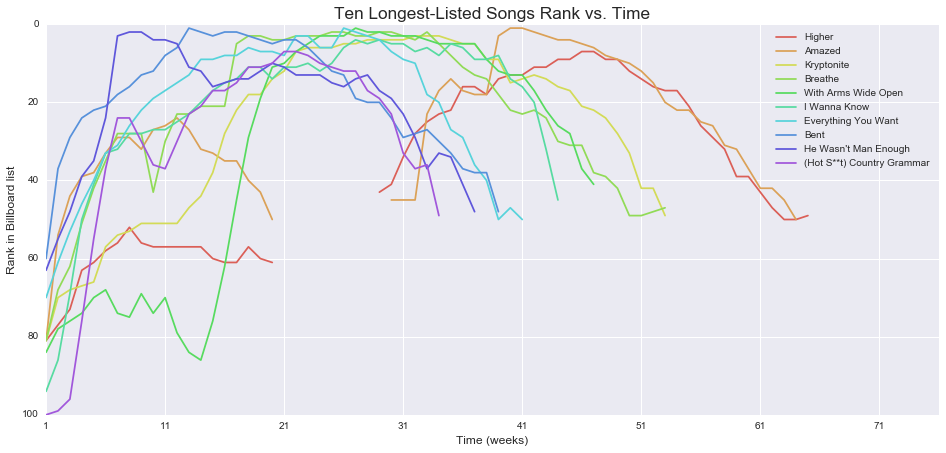
Songs that stayed the longest time on the billboard
# Find the songs that spent the most time on the Billboard
number_of_weeks = data.loc[:, 'x1st.week':'x76th.week'].count(axis = 1)
longest_stay_dataframe = data.merge(pd.DataFrame(data = number_of_weeks, columns = ['weeks_on_billboard']), left_index=True, right_index=True).sort_values(by = 'weeks_on_billboard', ascending = False)
#longest_stay_dataframe['weeks_on_billboard'] = number_of_weeks

# Sort by the number of weeks on the billboard
top_10_longest_stay_dataframe = longest_stay_dataframe[0:10]

top_10_longest_stay_dataframe[['track', 'artist_name', 'weeks_on_billboard']]
| track | artist_name | weeks_on_billboard | |
|---|---|---|---|
| 46 | Higher | Creed | 57 |
| 9 | Amazed | Lonestar | 55 |
| 24 | Kryptonite | 3 Doors Down | 53 |
| 17 | Breathe | Faith Hill | 53 |
| 13 | With Arms Wide Open | Creed | 47 |
| 28 | I Wanna Know | Joe | 44 |
| 12 | Everything You Want | Vertical Horizon | 41 |
| 15 | Bent | matchbox twenty | 39 |
| 20 | He Wasn't Man Enough | Toni Braxton | 37 |
| 47 | (Hot S**t) Country Grammar | Nelly | 34 |
Plotting how the top songs and the longest-staying songs moved
Let’s see how songs move on the billboard. We’ll look at the songs that reached #1 first, and then the songs that stayed on the billboard the longest.